Step 1

We are given the function ${y^2} = x$ and the dimension is $l = 2\;{\rm{m}}$ and $b = 4\;{\rm{m}}$.

We are asked to determine the product of inertia of the shaded area and then by using the parallel axis theorem calculate the product of inertia of the area with respect to the centroid.

 
Step 2

The coordinate diagram of the picture is shown below:

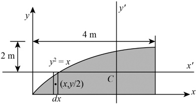
Since we know that the segment is symmetric so the differential moment of inertia is zero that is $d{I_0} = 0$.

The area of the surface is calculated as:

\[dA = ydx\]

The centroid of the segment about x-axis is,

\[\bar x = x\]

The centroid of the segment about y-axis is,

\[\bar y = \frac{y}{2}\]

To find the product of inertia of the shaded area about the $x - y$ axis we will use the parallel axis theorem.

\[d{I_{xy}} = d{I_0} + \left( {\bar x \times \bar y} \right)dA\]

Here, $\bar x$ and $\bar y$ are the centroid in $x$ and $y$ axis.

On plugging the values in the above relation, we get,

\[\begin{array}{l} d{I_{xy}} = 0 + \left( {x \times \frac{y}{2}} \right)\left( {ydx} \right)\\ d{I_{xy}} = \left( {x \times \frac{{{y^2}}}{2}} \right)dx\\ d{I_{xy}} = \left( {x \times \frac{x}{2}} \right)dx\\ d{I_{xy}} = \left( {\frac{{{x^2}}}{2}} \right)dx \end{array}\]
 
Step 3

On integrating the above relation, we get,

\[\begin{array}{l} {I_{xy}} = \int\limits_0^4 {\left( {\frac{{{x^2}}}{2}} \right)dx} \\ {I_{xy}} = \left( {\frac{{{x^3}}}{6}} \right)_0^4\\ {I_{xy}} = \left[ {\left( {\frac{{{{\left( {4\;{\rm{m}}} \right)}^3}}}{6}} \right) - \left( {\frac{0}{6}} \right)} \right]\\ {I_{xy}} = 10.66\;{{\rm{m}}^{\rm{4}}} \end{array}\]

To find the value of the area we will use the relation,

\[\begin{array}{l} \int {dA} = \int\limits_0^4 {ydx} \\ \int {dA} = \int\limits_0^4 {{x^{\left( {\frac{1}{2}} \right)}}dx} \\ \int {dA} = \left[ {\frac{{{x^{3/2}}}}{{\frac{3}{2}}}} \right]_0^4\\ \int {dA} = 5.33\;{{\rm{m}}^2} \end{array}\]

To find the x-coordinate of centroid of our area we will use the relation,

\[\begin{array}{l} \int {\bar xdA} = \int\limits_0^4 {xydx} \\ \int {\bar xdA} = \int\limits_0^4 {x \times {x^{\left( {\frac{1}{2}} \right)}}dx} \\ \int {\bar xdA} = \int\limits_0^4 {{x^{3/2}}dx} \end{array}\]

On integrating and plugging the values in the above relation, we get,

\[\begin{array}{l} \int {\bar xdA} = \left[ {\frac{{{x^{5/2}}}}{{\frac{5}{2}}}} \right]_0^4\\ \int {\bar xdA} = \left[ {\left( {\frac{{{{\left( {4\;{\rm{m}}} \right)}^{5/2}}}}{{\frac{5}{2}}}} \right) - \left( {\frac{{{{\left( {0\;{\rm{m}}} \right)}^{5/2}}}}{{\frac{5}{2}}}} \right)} \right]\\ \int {\bar xdA} = 12.8\;{{\rm{m}}^3} \end{array}\]
 
Step 4

To find the y-coordinate of centroid of our area we will use the relation,

\[\begin{array}{l} \int {\bar ydA} = \int\limits_0^4 {\left( {\frac{y}{2}} \right)ydx} \\ \int {\bar ydA} = \int\limits_0^4 {\frac{{{y^2}}}{2}dx} \end{array}\]

On integrating and plugging the values in the above relation, we get,

\[\begin{array}{l} \int {\bar ydA} = \int\limits_0^4 {\frac{x}{2}dx} \\ \int {\bar ydA} = \left[ {\frac{{{x^2}}}{4}} \right]_0^4\\ \int {\bar ydA} = \left[ {\left( {\frac{{{{\left( {4\;{\rm{m}}} \right)}^2}}}{4}} \right) - \left( {\frac{{{{\left( {0\;{\rm{m}}} \right)}^2}}}{4}} \right)} \right]\\ \int {\bar ydA} = 4\;{{\rm{m}}^3} \end{array}\]

To find the centroid of shaded area about x-axis we will use the relation,

\[{\bar x_0} = \frac{{\int {\bar xdA} }}{{\int {dA} }}\]

On plugging the values in the above relation, we get,

\[\begin{array}{l} {{\bar x}_0} = \left( {\frac{{12.8\;{{\rm{m}}^3}}}{{5.33\;{{\rm{m}}^2}}}} \right)\\ {{\bar x}_0} = 2.4\,{\rm{m}} \end{array}\]

To find the centroid of shaded area about y-axis we will use the relation,

\[{\bar y_0} = \frac{{\int {\bar ydA} }}{{\int {dA} }}\]

On plugging the values in the above relation, we get,

\[\begin{array}{l} {{\bar y}_0} = \left( {\frac{{4\;{{\rm{m}}^3}}}{{5.33\;{{\rm{m}}^2}}}} \right)\\ {{\bar y}_0} = 0.75\,{\rm{m}} \end{array}\]
 
Step 5

To find the product of inertia we will use the relation of parallel axis theorem,

\[I = {I_{xy}} - \left[ {{{\bar x}_0} \times {{\bar y}_0}\left( {dA} \right)} \right]\]

On plugging the values in the above relation, we get,

\[\begin{array}{l} I = \left( {10.66\;{{\rm{m}}^4}} \right) - \left[ {2.4\;{\rm{m}} \times 0.75\;{\rm{m}} \times {\rm{5}}{\rm{.33}}\;{{\rm{m}}^2}} \right]\\ I = 1.066\,{{\rm{m}}^4} \end{array}\]