Step 1

We are given the mass of a rod $m = 20\;{\rm{kg}}$, the coordinates of point $A$ as $A\left( {{x_a},{y_a},{z_a}} \right) = \left( {1.5,0,0} \right){\rm{m}}$, the coordinates of point $B$ as $B\left( {{x_b},{y_b},{z_b}} \right) = \left( {0,1,2} \right){\rm{m}}$, the coordinates of point $C$ as $C\left( {{x_c},{y_c},{z_c}} \right) = \left( {0,0,2.5} \right){\rm{m}}$.

We are asked to determine the reaction at $A$, the tension in the cable and the normal reaction at point $B$.

 
Step 2

We will draw a free body diagram of the rod.

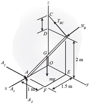
Here, ${A_x}$ is the reaction force at point $A$, ${A_y}$ is the reaction force at point $A$, ${A_z}$ is the reaction force at point $A$, and ${N_B}$ is the normal reaction force at point $B$.

 
Step 3

We will find the weight of the rod in vector form.

\[\begin{array}{l} {\bf{W}} = - W{\bf{k}}\\ {\bf{W}} = - \left( {mg} \right){\bf{k}} \end{array}\]

Here, $g = 9.81\;{\rm{m/}}{{\rm{s}}^{\rm{2}}}$ is the acceleration due to gravity.

Substitute the given value in the above equation.

\[\begin{array}{l} {\bf{W}} = - \left( {\left( {20\;{\rm{kg}}} \right)\left( {9.81\;{\rm{m/}}{{\rm{s}}^{\rm{2}}}} \right)} \right){\bf{k}}\\ = - \left( {\left( {196.2\;{\rm{kg}} \cdot {\rm{m/}}{{\rm{s}}^{\rm{2}}}} \right) \times \left( {\frac{{{\rm{1}}\;{\rm{N}}}}{{{\rm{1}}\;{\rm{kg}} \cdot {\rm{m/}}{{\rm{s}}^{\rm{2}}}}}} \right)} \right){\bf{k}}\\ = - \left( {{\rm{196}}{\rm{.2}}\;{\rm{N}}} \right){\bf{k}} \end{array}\]
 
Step 4

We will find the force vector at the joint $A$.

\[{{\bf{F}}_A} = - {A_x}{\bf{i}} + {A_y}{\bf{j}} + {A_z}{\bf{k}}\]
 
Step 5

We will find the normal reaction force at point $B$.

\[{{\bf{N}}_B} = {N_B}\left( {{\bf{i}} + 0{\bf{j}} + 0{\bf{k}}} \right)\]
 
Step 6

We will find the position vector $BC$.

\[\begin{array}{l} {{\bf{r}}_{BC}} = {{\bf{r}}_{OC}} - {{\bf{r}}_{OB}}\\ {{\bf{r}}_{BC}} = \left[ {\left( {{x_c} - 0} \right){\bf{i}} + \left( {{y_c} - 0} \right){\bf{j}} + \left( {{z_c} - 0} \right){\bf{k}}} \right] - \left[ {\left( {{x_b} - 0} \right){\bf{i}} + \left( {{y_b} - 0} \right){\bf{j}} + \left( {{z_b} - 0} \right){\bf{k}}} \right] \end{array}\]

Substitute the given value in the above equation.

\[\begin{array}{c} {{\bf{r}}_{BC}} = \left[ {\left( {0 - 0} \right){\bf{i}} + \left( {0 - 0} \right){\bf{j}} + \left( {2.5 - 0} \right){\bf{k}}} \right]{\rm{m}} - \left[ {\left( {0 - 0} \right){\bf{i}} + \left( {1 - 0} \right){\bf{j}} + \left( {2 - 0} \right){\bf{k}}} \right]{\rm{m}}\\ = \left[ {0{\bf{i}} + 0{\bf{j}} + 2.5{\bf{k}}} \right]{\rm{m}} - \left[ {0{\bf{i}} + 1{\bf{j}} + 2{\bf{k}}} \right]{\rm{m}}\\ = \left[ { - {\bf{j}} + 0.5{\bf{k}}} \right]{\rm{m}} \end{array}\]
 
Step 7

We will find the tension in the cable in vector form.

\[\begin{array}{l} {{\bf{T}}_{BC}} = {T_{BC}}\left( {\frac{{{{\bf{r}}_{BC}}}}{{{r_{BC}}}}} \right)\\ {{\bf{T}}_{BC}} = {T_{BC}}\left( {\frac{{{{\bf{r}}_{BC}}}}{{\sqrt {{{\left( {{r_{BCy}}} \right)}^2} + {{\left( {{r_{BCz}}} \right)}^2}} }}} \right) \end{array}\]

Here, ${r_{BC}}$ is the magnitude of the position vector, ${r_{BCy}} = - {\rm{1}}\;{\rm{m}}$ isthe $y$ component, and ${r_{BCz}} = 0.{\rm{5}}\;{\rm{m}}$ is the $z$ component.

Substitute the given value in the above equation.

\[\begin{array}{c} {{\bf{T}}_{BC}} = {T_{BC}}\left( {\frac{{\left[ { - {\bf{j}} + 0.5{\bf{k}}} \right]{\rm{m}}}}{{\sqrt {{{\left( { - 1\;{\rm{m}}} \right)}^2} + {{\left( {{\rm{0}}{\rm{.5}}\;{\rm{m}}} \right)}^2}} }}} \right)\\ = {T_{BC}}\left( {\frac{{\left[ { - {\bf{j}} + 0.5{\bf{k}}} \right]}}{{\sqrt {1.25} }}} \right)\\ = \left( { - \frac{1}{{\sqrt {1.25} }}{T_{BC}}} \right){\bf{j}} + \left( {\frac{{0.5}}{{\sqrt {1.25} }}{T_{BC}}} \right){\bf{k}} \end{array}\]
 
Step 8

We will find the position vector $AB$.

\[\begin{array}{l} {{\bf{r}}_{AB}} = {{\bf{r}}_{OB}} - {{\bf{r}}_{OA}}\\ {{\bf{r}}_{AB}} = \left[ {\left( {{x_b} - 0} \right){\bf{i}} + \left( {{y_b} - 0} \right){\bf{j}} + \left( {{z_b} - 0} \right){\bf{k}}} \right] - \left[ {\left( {{x_a} - 0} \right){\bf{i}} + \left( {{y_a} - 0} \right){\bf{j}} + \left( {{z_a} - 0} \right){\bf{k}}} \right] \end{array}\]

Substitute the given value in the above equation.

\[\begin{array}{c} {{\bf{r}}_{AB}} = \left[ {\left( {0 - 0} \right){\bf{i}} + \left( {1 - 0} \right){\bf{j}} + \left( {2 - 0} \right){\bf{k}}} \right]{\rm{m}} - \left[ {\left( {1.5 - 0} \right){\bf{i}} + \left( {0 - 0} \right){\bf{j}} + \left( {0 - 0} \right){\bf{k}}} \right]{\rm{m}}\\ = \left[ {0{\bf{i}} + 1{\bf{j}} + 2{\bf{k}}} \right]{\rm{m}} - \left[ {1.5{\bf{i}} + 0{\bf{j}} + 0{\bf{k}}} \right]{\rm{m}}\\ = \left[ { - 1.5{\bf{i}} + 1{\bf{j}} + 2{\bf{k}}} \right]{\rm{m}} \end{array}\]
 
Step 9

We will find the position vector $AG$.

\[{{\bf{r}}_{AG}} = \frac{1}{2}{{\bf{r}}_{AB}}\]

Substitute the given value in the above equation.

\[\begin{array}{c} {{\bf{r}}_{AG}} = \frac{1}{2}{{\bf{r}}_{AB}}\\ = \frac{1}{2}\left[ { - 1.5{\bf{i}} + 1{\bf{j}} + 2{\bf{k}}} \right]{\rm{m}}\\ = \left[ { - 0.75{\bf{i}} + 0.5{\bf{j}} + {\bf{k}}} \right]{\rm{m}} \end{array}\]
 
Step 10

We will take the moment about point $A$.

\[\begin{array}{c} \sum {{M_A}} = 0\\ {r_{AG}} \times W + \left[ {{r_{AB}} \times \left( {{T_{BC}} + {N_B}} \right)} \right] = 0 \end{array}\]

Substitute the given value in the above equation.

\[\begin{array}{c} \left[ \begin{array}{l} \left[ { - 0.75{\bf{i}} + 0.5{\bf{j}} + {\bf{k}}} \right]{\rm{m}} \times \left( { - \left( {{\rm{196}}{\rm{.2}}\;{\rm{N}}} \right){\bf{k}}} \right) + \\ \left[ {\left[ { - 1.5{\bf{i}} + 1{\bf{j}} + 2{\bf{k}}} \right]{\rm{m}} \times \left( {\left[ {\left( { - \frac{1}{{\sqrt {1.25} }}{T_{BC}}} \right){\bf{j}} + \left( {\frac{{0.5}}{{\sqrt {1.25} }}{T_{BC}}} \right){\bf{k}}} \right] + \left[ {{N_B}\left( {{\bf{i}} + 0{\bf{j}} + 0{\bf{k}}} \right)} \right]} \right)} \right] \end{array} \right] = 0\\ \left| {\begin{array}{*{20}{c}} {\bf{i}}&{\bf{j}}&{\bf{k}}\\ { - 0.75}&{0.5}&1\\ 0&0&{ - 196.2} \end{array}} \right| + \left| {\begin{array}{*{20}{c}} {\bf{i}}&{\bf{j}}&{\bf{k}}\\ { - 1.5}&1&2\\ {{N_B}}&{ - \frac{1}{{\sqrt {1.25} }}{T_{BC}}}&{\frac{{0.5}}{{\sqrt {1.25} }}{T_{BC}}} \end{array}} \right| = 0 \end{array}\]

Solve the above equation.

\[\begin{array}{c} \left[ \begin{array}{l} \left[ {\left( {0.5 \times \left( { - 196.2} \right) - 0 \times 1} \right){\bf{i}} - \left( { - 0.75 \times \left( { - 196.2} \right) - 0 \times 1} \right){\bf{j}} + \left( { - 0.75 \times 0 - 0 \times 0.5} \right){\bf{k}}} \right] + \\ \left[ \begin{array}{l} \left( {1 \times \left( {\frac{{0.5}}{{\sqrt {1.25} }}{T_{BC}}} \right) - \left( { - \frac{1}{{\sqrt {1.25} }}{T_{BC}}} \right) \times 2} \right){\bf{i}} - \left( { - 1.5 \times \left( {\frac{{0.5}}{{\sqrt {1.25} }}{T_{BC}}} \right) - {N_B} \times 2} \right){\bf{j}} + \\ \left( { - 1.5 \times \left( { - \frac{1}{{\sqrt {1.25} }}{T_{BC}}} \right) - {N_B} \times 1} \right){\bf{k}} \end{array} \right] \end{array} \right] = 0\\ \left[ {\left[ { - 98.1{\bf{i}} - 147.15{\bf{j}}} \right] + \left[ \begin{array}{l} \left( {\frac{{0.5}}{{\sqrt {1.25} }}{T_{BC}} + \frac{2}{{\sqrt {1.25} }}{T_{BC}}} \right){\bf{i}} + \left( {\frac{{0.75}}{{\sqrt {1.25} }}{T_{BC}} + 2{N_B}} \right){\bf{j}} + \\ \left( {\frac{{1.5}}{{\sqrt {1.25} }}{T_{BC}} - {N_B}} \right){\bf{k}} \end{array} \right]} \right] = 0\\ \left[ {\left( {\frac{{0.5}}{{\sqrt {1.25} }}{T_{BC}} + \frac{2}{{\sqrt {1.25} }}{T_{BC}} - 98.1} \right){\bf{i}} + \left( {\frac{{0.75}}{{\sqrt {1.25} }}{T_{BC}} + 2{N_B} - 147.15} \right){\bf{j}} + \left( {\frac{{1.5}}{{\sqrt {1.25} }}{T_{BC}} - {N_B}} \right){\bf{k}}} \right] = 0 \end{array}\]
 
Step 11

Compare the ${\bf{i}},{\bf{j}}$ and ${\bf{k}}$ components.

\[\frac{{0.5}}{{\sqrt {1.25} }}{T_{BC}} + \frac{2}{{\sqrt {1.25} }}{T_{BC}} - 98.1 = 0\;\;\;\;...\left( 1 \right)\] \[\frac{{0.75}}{{\sqrt {1.25} }}{T_{BC}} + 2{N_B} - 147.15 = 0\;\;\;\;\;\;\;\;\;...\left( 2 \right)\] \[\begin{array}{c} \left( {\frac{{1.5}}{{\sqrt {1.25} }}{T_{BC}} - {N_B}} \right) = 0\\ {N_B} = \frac{{1.5}}{{\sqrt {1.25} }}{T_{BC}}\;\;\;\;\;\;\;\;\;\;\;\;\;\;...\left( 3 \right) \end{array}\]
 
Step 12

We will solve the equation (3) and (2) to find the tension in the cable $BC$.

\[\begin{array}{c} \frac{{0.75}}{{\sqrt {1.25} }}{T_{BC}} + 2{N_B} - 147.15 = 0\\ \frac{{0.75}}{{\sqrt {1.25} }}{T_{BC}} + 2\left( {\frac{{1.5}}{{\sqrt {1.25} }}{T_{BC}}} \right) - 147.15 = 0\\ {T_{BC}}\left( {\frac{{3.75}}{{\sqrt {1.25} }}} \right) = 147.15\\ {T_{BC}} = \frac{{147.15}}{{\left( {\frac{{3.75}}{{\sqrt {1.25} }}} \right)}}\\ \approx 43.9\;{\rm{N}} \end{array}\]
 
Step 13

Substitute the given value in equation (3) to find the normal reaction at point $B$.

\[\begin{array}{c} {N_B} = \frac{{1.5}}{{\sqrt {1.25} }} \times \left( {{\rm{43}}{\rm{.9}}\;{\rm{N}}} \right)\\ \approx 58.9\;{\rm{N}} \end{array}\]
 
Step 14

We will apply the force equilibrium condition.

\[\begin{array}{r} \sum F = 0\\ {{\bf{F}}_A} + {{\bf{T}}_{BC}} + {{\bf{N}}_B} + {\bf{W}} = 0 \end{array}\]

Substitute the given value in the above equation.

\[\begin{array}{c} \left[ { - {A_x}{\bf{i}} + {A_y}{\bf{j}} + {A_z}{\bf{k}}} \right] + \left[ {\left( { - \frac{1}{{\sqrt {1.25} }}{T_{BC}}} \right){\bf{j}} + \left( {\frac{{0.5}}{{\sqrt {1.25} }}{T_{BC}}} \right){\bf{k}}} \right] + {N_B}\left( {{\bf{i}} + 0{\bf{j}} + 0{\bf{k}}} \right) + \left[ { - \left( {{\rm{196}}{\rm{.2}}\;{\rm{N}}} \right){\bf{k}}} \right] = 0\\ \left( { - {A_x} + {N_B}} \right){\bf{i}} + \left( {{A_y} - \frac{1}{{\sqrt {1.25} }}{T_{BC}}} \right){\bf{j}} + \left( {{A_z} + \frac{{0.5}}{{\sqrt {1.25} }}{T_{BC}} - {\rm{196}}{\rm{.2}}\;{\rm{N}}} \right){\bf{k}} = 0 \end{array}\] Step 15

Compare the ${\bf{i}},{\bf{j}}$ and ${\bf{k}}$ components.

\[ - {A_x} + {N_B} = 0\;\;\;\;\;\;\;\;\;\;\;\;\;...\left( 4 \right)\] \[{A_y} - \frac{1}{{\sqrt {1.25} }}{T_{BC}} = 0\;\;\;\;\;\;\;\;\;...\left( 5 \right)\] \[{A_z} + \frac{{0.5}}{{\sqrt {1.25} }}{T_{BC}} - {\rm{196}}{\rm{.2}}\;{\rm{N}} = 0\;\;\;\;\;\;...\left( 6 \right)\]
 
Step 16

Substitute the given value in equation (4) to find the reaction at point $A$ along the $x$ axis.

\[\begin{array}{c} - {A_x} + 58.9\;{\rm{N}} = 0\\ {A_x} = 58.9\;{\rm{N}} \end{array}\]
 
Step 17

Substitute the given value in equation (5) to find the reaction at point $A$ along the $y$ axis.

\[\begin{array}{c} {A_y} - \frac{1}{{\sqrt {1.25} }} \times \left( {43.9\;{\rm{N}}} \right) = 0\\ {A_y} = \frac{1}{{\sqrt {1.25} }} \times \left( {43.9\;{\rm{N}}} \right)\\ \approx 39.3\;{\rm{N}} \end{array}\]
 
Step 18

Substitute the given value in equation (6) to find the reaction at point $A$ along the $z$ axis.

\[\begin{array}{c} {A_z} + \frac{{0.5}}{{\sqrt {1.25} }} \times \left( {43.9\;{\rm{N}}} \right) - {\rm{196}}{\rm{.2}}\;{\rm{N}} = {\rm{0}}\\ {A_z} = {\rm{196}}{\rm{.2}}\;{\rm{N}} - \frac{{0.5}}{{\sqrt {1.25} }} \times \left( {43.9\;{\rm{N}}} \right)\\ \approx 176.6\;{\rm{N}} \end{array}\]