Step 1

We are given that the equation of first curve is ${y_1} = - x$ and the equation of second curve is ${y_2} = \sqrt {2x} $. The thickness of plate is $t = 0.3\;{\rm{m}}$ and the density of plate is $\rho = 7850\;{\rm{kg/}}{{\rm{m}}^3}$.

We are asked to locate the center of mass of plate and the reactions at the pin and roller support.

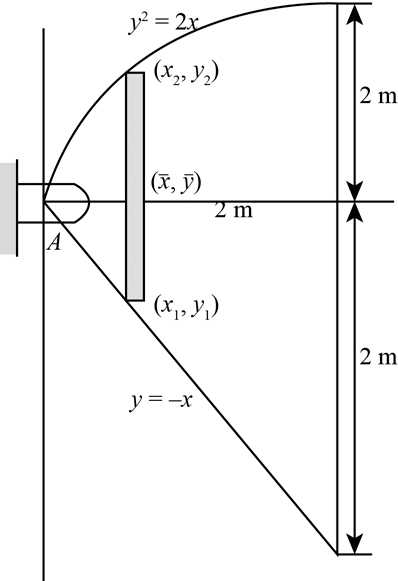
We have the vertical distance of first curve from axis is ${h_1} = 2\;{\rm{m}}$.

We have the vertical distance of second curve from axis is ${h_2} = 2\;{\rm{m}}$.

We have the horizontal distance of point A to end point is $d = 2\;{\rm{m}}$.

 
Step 2

The centroid of the given curves is given as:

\[\left( {\bar x,\bar y} \right) = \left( {x,\frac{{{y_1} + {y_2}}}{2}} \right)\]
 
Step 3

To calculate the area of strip we use the formula:

\[dA = \left( {{y_2} - {y_1}} \right)dx\]
 
Step 4

Substitute the known values in the formula:

\begin{array}{c} dA = \left( {\sqrt {2x} - \left( { - x} \right)} \right)dx\\ = \left( {\sqrt {2x} + x} \right)dx \end{array}
 
Step 5

To calculate the centroid of curve about x-axis we use the formula:

\[\bar x = \frac{{\int {\bar xdA} }}{{\int {dA} }}\]...... (1)
 
Step 6

The numerator of the equation (1) is calculated as:

\begin{array}{c} \int {\bar xdA} = \int\limits_0^2 {x\left( {\sqrt {2x} + x} \right)dx} \\ = \int\limits_0^2 {\left( {\sqrt 2 {x^{3/2}} + {x^2}} \right)dx} \\ = \left[ {\sqrt 2 \frac{{{x^{5/2}}}}{{\left( {\frac{5}{2}} \right)}} + \frac{{{x^3}}}{3}} \right]_0^2\\ = \left[ {\frac{{2\sqrt 2 }}{5}{x^{5/2}} + \frac{{{x^3}}}{3}} \right]_0^2 \end{array}
 
Step 7

Substitute the lower and upper limit of integration in the equation:

\[\begin{array}{c} \int {\bar x} dA = \left( {\frac{{2\sqrt 2 }}{5}{{\left( 2 \right)}^{5/2}} + \frac{{{{\left( 2 \right)}^3}}}{3}} \right) - \left( {\frac{{2\sqrt 2 }}{5}{{\left( 0 \right)}^{5/2}} + \frac{{{{\left( 0 \right)}^3}}}{3}} \right)\\ = \left( {3.2 + 2.67} \right) - \left( {0 + 0} \right)\\ = 5.87 \end{array}\]
 
Step 8

The denominator of the equation (1) is calculated as:

\begin{array}{c} \int {dA} = \int\limits_0^2 {\left( {\sqrt {2x} + x} \right)dx} \\ = \left[ {\frac{{\sqrt 2 {x^{3/2}}}}{{\left( {\frac{3}{2}} \right)}} + \frac{{{x^2}}}{2}} \right]_0^2\\ = \left[ {\frac{{2\sqrt 2 {x^{3/2}}}}{3} + \frac{{{x^2}}}{2}} \right]_0^2 \end{array}
 
Step 9

Substitute the lower and upper limit of integration in the equation:

\begin{array}{c} \int {dA} = \left( {\frac{{2\sqrt 2 {{\left( 2 \right)}^{3/2}}}}{3} + \frac{{{{\left( 2 \right)}^2}}}{2}} \right) - \left( {\frac{{2\sqrt 2 {{\left( 0 \right)}^{3/2}}}}{3} + \frac{{{{\left( 0 \right)}^2}}}{2}} \right)\\ = 2.667 + 2\\ = 4.667 \end{array}
 
Step 10

Substitute the known values in equation (1):

\begin{array}{c} \bar x = \frac{{5.87}}{{4.667}}\\ = 1.26 \end{array}Step 11

To calculate the centroid of curve about y-axis we use the formula:

\[\bar y = \frac{{\int {\bar ydA} }}{{\int {dA} }}\]...... (2)
 
Step 12

The numerator of the equation (2) is calculated as:

\[\int {\bar ydA} = \int\limits_0^2 {\left( {\frac{{{y_1} + {y_2}}}{2}} \right)\left( {\sqrt {2x} + x} \right)dx} \]
 
Step 13

Substitute the known values in equation:

\begin{array}{c} \int {\bar y} dA = \int\limits_0^2 {\left( {\frac{{ - x + \sqrt {2x} }}{2}} \right)\left( {\sqrt {2x} + x} \right)dx} \\ = \frac{1}{2}\int\limits_0^2 {\left( {{{\left( {\sqrt {2x} } \right)}^2} - {{\left( x \right)}^2}} \right)} dx\\ = \frac{1}{2}\left[ {\frac{{2{x^2}}}{2} - \frac{{{x^3}}}{3}} \right]_0^2\\ = \frac{1}{2}\left[ {{x^2} - \frac{{{x^3}}}{3}} \right]_0^2 \end{array}
 
Step 14

Substitute the lower and upper limit of integration in the equation:

\begin{array}{c} \int {\bar y} dA = \frac{1}{2}\left( {{{\left( 2 \right)}^2} - \frac{{{{\left( 2 \right)}^3}}}{3}} \right) - \frac{1}{2}\left( {{{\left( 0 \right)}^2} - \frac{{{{\left( 0 \right)}^3}}}{3}} \right)\\ = \frac{1}{2}\left( {4 - 2.67} \right) - \frac{1}{2}\left( {0 - 0} \right)\\ = \frac{1}{2}\left( {1.33} \right)\\ = 0.665 \end{array}
 
Step 15

Substitute the known values in equation (2):

\begin{array}{c} \bar y = \frac{{0.665}}{{4.667}}\\ = 0.142 \end{array}
 
Step 16

To calculate the weight of the plate we use the formula:

\[W = \rho gAt\]
 
Step 17

Substitute the known values in the formula:

\begin{array}{c} W = \left( {7850\;{\rm{kg/}}{{\rm{m}}^3}} \right)\left( {9.81\;{\rm{m/}}{{\rm{s}}^2}} \right)\left( {4.667\;{{\rm{m}}^2}} \right)\left( {0.3\;{\rm{m}}} \right)\left( {\frac{{1\;{\rm{N}}}}{{1\;{\rm{kg}} \cdot {\rm{m/}}{{\rm{s}}^2}}}} \right)\\ = 107819.6\;{\rm{N}} \end{array}
 
Step 18

The free body diagram of the plate is shown as:

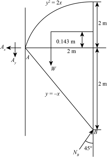
Here, ${A_x}$ is the reaction at point A, ${A_y}$ is the reaction at point A and ${N_B}$ is the normal force at point B which makes an angle $\theta = 45^\circ $.

 
Step 19

Applying the moment of force equation about point A:

\[ - \bar xW + {N_B}\cos \theta {h_2} + {N_B}\sin \theta d = 0\]
 
Step 20

Substitute the known values in the equation:

\[\begin{array}{c} \left\{ \begin{array}{l} - \left( {1.26\;{\rm{m}}} \right)\left( {107819.6\;{\rm{N}}} \right) + \\ {N_B}\cos 45^\circ \left( {2\;{\rm{m}}} \right) + \\ {N_B}\sin 45^\circ \left( {2\;{\rm{m}}} \right) \end{array} \right\} = 0\\ {N_B}\left( {\left( {0.707} \right)\left( {2\;{\rm{m}}} \right) + \left( {0.707} \right)\left( {2\;{\rm{m}}} \right)} \right) = {\rm{135852}}{\rm{.7}}\;{\rm{N}}\\ {N_B} = \frac{{{\rm{135852}}{\rm{.7}}\;{\rm{N}}}}{{2.828}}\\ = {\rm{48038}}{\rm{.4}}\;{\rm{N}} \end{array}\]
 
Step 21

Applying the equilibrium force of equation along x-axis:

\begin{array}{c} \sum {F_x} = 0\\ - {A_x} + {N_B}\sin \theta = 0 \end{array}
 
Step 22

Substitute the known values in the equation:

\[\begin{array}{c} - {A_x} + \left( {48038.4\;{\rm{N}}} \right)\sin 45^\circ = 0\\ {A_x} = \left( {48038.4\;{\rm{N}}} \right)\left( {0.707} \right)\\ = {\rm{33963}}{\rm{.1}}\;{\rm{N}} \end{array}\]
 
Step 23

Applying the equilibrium force of equation along y-axis:

\begin{array}{c} \sum {F_y} = 0\\ {A_y} + {N_B}\cos \theta - W = 0 \end{array}
 
Step 24

Substitute the known values in the equation:

\[\begin{array}{c} \left\{ \begin{array}{l} {A_y} + \left( {48038.4\;{\rm{N}}} \right)\cos 45^\circ \\ - 107819.6\;{\rm{N}} \end{array} \right\} = 0\\ {A_y} = - \left( {48038.4\;{\rm{N}}} \right)\left( {0.707} \right) + 107819.6\;{\rm{N}}\\ = - {\rm{33963}}{\rm{.1}}\;{\rm{N}} + 107819.6\;{\rm{N}}\\ = {\rm{73856}}{\rm{.5}}\;{\rm{N}} \end{array}\]