Step 1

The accompanying data on the residual flame time for the strips of treated children’s nightwear are provided. A true average flame time of at most 9.75 has been fixed.

 
Step 2

It is to be tested that the true average flame time for strips of the treated children’s nightwear is more than 9.75 at 5% level of significance.

Let $\mu $ be the true average flame time for strips of the treated children’s nightwear. The hypotheses become:

\[\begin{array}{l} {H_o}\,:\,\mu = \,9.75\\ {H_1}\,:\,\mu > \,9.75 \end{array}\]

The one-sample t test statistic will be used;

\[t\, = \,\frac{{\left( {\bar x\, - \,{\mu _ \circ }} \right)}}{{\frac{s}{{\sqrt n }}}}\]

The one-sample t test is used under the basic assumption that data should be normally distributed, hence, a normal probability plot can be plotted.

Look at the normal probability plot which is obtained by plotting the X-values (sample data) on the horizontal axis, and the corresponding percent on your vertical axis.

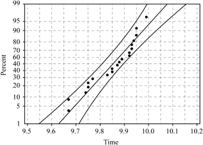
If the given data points on the plot cluster close to the straight line, then, the sample distribution attains normality.

From the plot, it is clear that distribution follows approximately normal distribution. Therefore, t-test can be used.

 
Step 3

The calculation for the given data in tabular form;

SL. No	x	\[{\left( {{x_i} - \,\bar x} \right)^2}\]
1	9.85	6.25E-06
2	9.94	0.007656
3	9.88	0.000756
4	9.93	0.006006
5	9.85	6.25E-06
6	9.95	0.009506
7	9.75	0.010506
8	9.75	0.010506
9	9.95	0.009506
10	9.77	0.006806
11	9.83	0.000506
12	9.93	0.006006
13	9.67	0.033306
14	9.92	0.004556
15	9.92	0.004556
16	9.87	0.000306
17	9.74	0.012656
18	9.89	0.001406
19	9.67	0.033306
20	9.99	0.018906
Total	197.05	0.176775

Mean of flame time is;

\[\begin{array}{c} \bar x\, = \,\frac{{197.5}}{{20}}\\ = \,9.8525 \end{array}\]

Standard deviation of flame time is;

\[\begin{array}{c} s\, = \,\sqrt {\frac{{\sum {{{\left( {{x_i} - \,\bar x} \right)}^2}} }}{{n - 1}}} \\ = \sqrt {\frac{{0.176775}}{{19}}} \\ = \,0.096457 \end{array}\]

On substitution, t-statistic becomes;

\[\begin{array}{c} t\, = \,\frac{{\left( {9.8525\, - \,9.75} \right)}}{{\frac{{0.096457}}{{\sqrt {20} }}}}\\ = \,\frac{{0.1025}}{{\frac{{0.02157}}{{\sqrt {20} }}}}\\ = \,4.7523 \end{array}\]

The test statistic is 4.7523.

Use the t-distribution table, at the 0.05 level of significance, the critical value for 19 degrees of freedom is 1.7291 which is less than the test statistic value. Hence, null hypothesis can be rejected.

Thus, there is solid evidence that the true average flame time for strips of the treated children’s nightwear more than 9.75 at 05% level of significance.